User Interface
There are two option to visualize gene expression on ClockProfile for individual genes (search by genes) and for gene sets (search by gene set).
search by gene (main gene view)
In the search by gene, the user has several options to view the data. Genes can be added and deleted in the search pane. All selected genes can be visualized in different ways:
- Rhythmicity plot (classic)
This plot is suitable to visualize up to 24 genes. All samples are represented by points at the respective sampling time (Zeitgeber Time (ZT) in h). ZT is the time in h after the light has been switched on.
Available options for this plot type on the search pane include: Log Scale: Select to represent the expression on a logarithmic scale Hide fit curve: Select to display the inferred fit on selected gene expression Scale fixed: Select to match the scale of the y-axis between all displayed mouse models
- Rhythmicity plot (radar)
This view represents each gene as one point in a radar plot for each indicated mouse model (i.e. Cry1+/+/Cry2+/+, Cry1-/-/Cry2-/-, Bmal1+/+, Bmal1-/-, Hlf+/+/Dbp+/+/Tef+/+, and Hlf-/-/Dbp-/-/Tef-/-). This plot is suitable to visualize several genes at once as amplitude and phase are condensed in one point for each mouse model.
Available options for this plot type on the search pane: Show change line: Select to display amplitude and phase for the respective KO or WT model
-
Mean differences
This plot shows the differential mean expression between the KO and WT siblings.
- Summary table
The table summarizes the computed parameters and selected models including the statistics for each gene. Table is sortable with a click on . Hold CTR and select if you want to sort several columns.

NRF rhythm: Color represent shared parameters (i.e. amplitude, phase) between different conditions BWT (Bmal1+/+), CWT (Cry1+/+/Cry2+/+), BKO (Bmal1-/-), CKO (Cry1-/--/-) under a night restricted feeding (NRF) regimen.
- Model:chosen model with highest BICW for rhythmic expression. To display BICW values of alternative models for the selected gene clock on the BICW value.
- BICW: Bayesian information criteria weight. See paragraph Bayesian information criteria weight for more details (below).
- Class: Genes classified according to their rhythmic expression pattern.
NRF mean: Color represent shared mean between different conditions: BWT (Bmal1+/+), CWT (Cry1+/+/Cry2+/+), BKO (Bmal1-/-), CKO (Cry1-/-/Cry2-/-)
- Model: chosen model with highest BICW for mean expression. To display BICW values of alternative models for the selected gene click on the BICW value.
- BICW: Bayesian information criteria weight. See paragraph Bayesian information criteria weight for more details (below).
- Class: Genes classified according to their Log2 fold change between KO and WT for Bmal1 and Cry1/2 mouse models.
PAR bZIp rhythm: Color represent shared parameters (i.e. amplitude, phase) between WT (Hlf+/+/Dbp+/+/Tef+/+) and KO (Hlf-/-/Dbp-/-/Tef-/-).
- Model: chosen model with highest BICW for rhythmic expression. To display BICW values of alternative models for the selected gene click on the BICW value.
- BICW: Bayesian information criteria weight. See paragraph Bayesian information criteria weight for more details (below).
PAR bZIp mean: Color represent shared mean (i.e. amplitude, phase) between different WT (Hlf+/+/Dbp+/+/Tef+/+) and KO (Hlf-/-/Dbp-/-/Tef-/-).
- Model: chosen model with highest BICW for mean expression. To display BICW values of alternative models for the selected gene click on the BICW value.
- BICW: Bayesian information criteria weight. See paragraph Bayesian information criteria weight for more details (below).
-
Download
Expression data and statistics can be downloaded for all selected genes for Bmal1 KO and Cry1/2 dKO dataset (NRF) and the Hlf/Dbp/Tef tKO mice dataset (PAR bZIp KO).
search by geneset
In this query mode. All expressed genes in mouse liver are grouped in functional gene sets. In the search by gene set, the user has several options to view the data.
- Go back to main view
After a gene set has been selected all genes of the selected gene set are shown in a table. The user can select or deselect genes of the table. By clicking on "go back to main view" the selected genes will be visualized as outlined search by gene (main gene view).
-
Mean enrichment
All genes belonging to the selected gene set are displayed in the left graph. Enrichment analysis are represented as -Log(p-value) for the indicated class of mean differences (right barplot).
- Phase enrichment
All rhythmic genes of the selected gene set are visualized in the left radar plot. The gene set enrichment is shown for each Zeitgeber time for the indicated class of genes.
Experimental setup
Male mice were kept under diurnal lighting conditions (12-hr light 12-hr dark). Mouse KO models for the core clock genes Bmal1 and Cry1/2 had restricted access to a chow diet during their activity period 4 day before sacrifice. All mice used in the experiments were between 9 and 14 weeks old. Genetical background and the generation of Bmal1 KO and Cry1/2 dKO have been previously described in Jouffe et al. [1]. The utilized PAR bZIP KO mouse models were described in detail in Gachon et al. [2]. These animals were fed ad libitum as feeding rhythms were not different to wild-type siblings.
RNA-Seq
Raw files and technical details about the RNA-Seq data have been deposited in NCBI's Gene Expression Omnibus [3] and are accessible through GEO Series accession number GSE135898 (https://www.ncbi.nlm.nih.gov/geo/query/acc.cgi?acc=GSE135898) and GSE135875 (https://www.ncbi.nlm.nih.gov/geo/query/acc.cgi?acc=GSE135875).
Modeling temporal gene expression profiles across different conditions
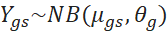
To assess rhythmicity and mean differences of gene expression in RNA-Seq count data, we developed a model selection framework based on generalized linear models. As proposed [4], we modeled counts ![]() that have been uniquely mapped to a gene
that have been uniquely mapped to a gene ![]() in a sample s as a negative binomial (NB) with a fitted mean
in a sample s as a negative binomial (NB) with a fitted mean ![]() and a gene-specific but sample-independent dispersion parameter
and a gene-specific but sample-independent dispersion parameter ![]() .
.
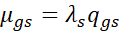
The fitted mean is proportional to the quantity ![]() of fragments that correspond to a gene g in a sample
of fragments that correspond to a gene g in a sample ![]() scaled by a sample-specific scaling factor
scaled by a sample-specific scaling factor ![]() [4]. This scaling factor depends on the sampling depth of each library and was estimated using the median-of-ratios method of DESeq2 [5].
[4]. This scaling factor depends on the sampling depth of each library and was estimated using the median-of-ratios method of DESeq2 [5].
A gene-specific distribution ![]() was estimated using empirical Bayes shrinkage [4].
was estimated using empirical Bayes shrinkage [4].
The fit was performed using a generalized linear model (GLM) with a logarithmic link function implemented in DESeq2. Sample specific size factor (![]() ) was defined as an offset. The full GLM was defined as follows:
) was defined as an offset. The full GLM was defined as follows:

where ![]() is the mean of the NB distribution for gene
is the mean of the NB distribution for gene ![]() and condition
and condition ![]() in sample
in sample ![]() at Zeitgeber/circadian time . The index
at Zeitgeber/circadian time . The index ![]() refers to a batch of samples. The parameters
refers to a batch of samples. The parameters ![]() and
and ![]() are coefficients of the cosine and sine functions, respectively.
are coefficients of the cosine and sine functions, respectively. ![]() is a coefficient to describe a condition specific mean expression level. When necessary, we included a batch specific
is a coefficient to describe a condition specific mean expression level. When necessary, we included a batch specific ![]() to account for technical batch effects. To select an optimal gene-specific model, we proceeded in two steps. First, we assessed rhythmicity across the different conditions, where the parameters
to account for technical batch effects. To select an optimal gene-specific model, we proceeded in two steps. First, we assessed rhythmicity across the different conditions, where the parameters ![]() and
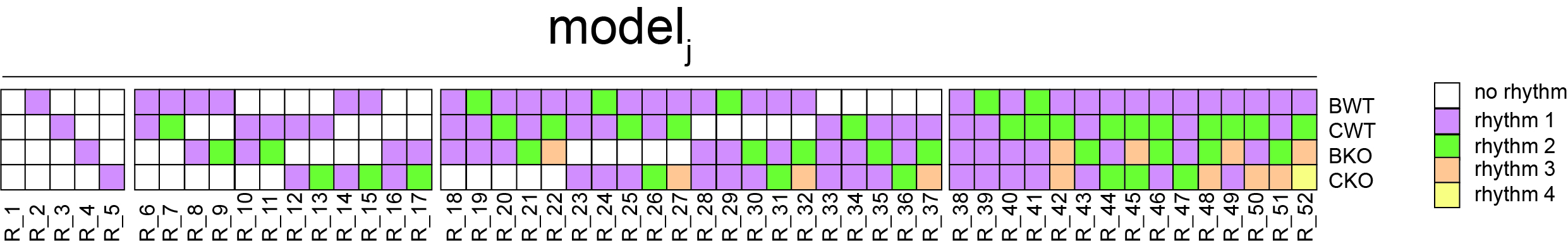
and ![]() were free but the parameters and had constraints depending on the particular model considered. To this end, we defined different models for four (e.g., Bmal1 WT, Bmal1 KO, Cry1/2 WT, Cry1/2 KO) or two conditions (i.e., PARbZip deficient (Hlf/Dbp/Tef KO) and proficient (Hlf/Dbp/Tef WT). Models were defined to have either zero (non-rhythmic pattern) or non-zero (rhythmic pattern)
were free but the parameters and had constraints depending on the particular model considered. To this end, we defined different models for four (e.g., Bmal1 WT, Bmal1 KO, Cry1/2 WT, Cry1/2 KO) or two conditions (i.e., PARbZip deficient (Hlf/Dbp/Tef KO) and proficient (Hlf/Dbp/Tef WT). Models were defined to have either zero (non-rhythmic pattern) or non-zero (rhythmic pattern) ![]() and
and ![]() coefficients for each analyzed condition. Moreover, for some models the values of
coefficients for each analyzed condition. Moreover, for some models the values of ![]() and
and ![]() can be also shared within any combination of the four conditions. For example, for four conditions, there are 52 such models (figure below). The coefficients
can be also shared within any combination of the four conditions. For example, for four conditions, there are 52 such models (figure below). The coefficients ![]() and
and ![]() were used to calculate the phase (
were used to calculate the phase (![]() ) and amplitude (log2-fold change peak-to-trough;
) and amplitude (log2-fold change peak-to-trough; ![]() ) of a gene. Bayesian information criterion (BIC) based model selection was employed to account for model complexity [6] using the following formula:
) of a gene. Bayesian information criterion (BIC) based model selection was employed to account for model complexity [6] using the following formula:
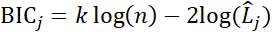
![]() is defined as the log-likelihood of the model j from the regression, n is the number of data points and k is the number of parameters. To assess the confidence of the selected model j we calculated the Schwarz weight (BICW):
is defined as the log-likelihood of the model j from the regression, n is the number of data points and k is the number of parameters. To assess the confidence of the selected model j we calculated the Schwarz weight (BICW):
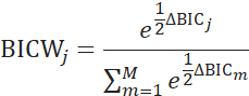
, where ![]() is defined as the difference in BIC between model j and the minimum BIC value in the entire model set
is defined as the difference in BIC between model j and the minimum BIC value in the entire model set ![]()
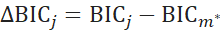
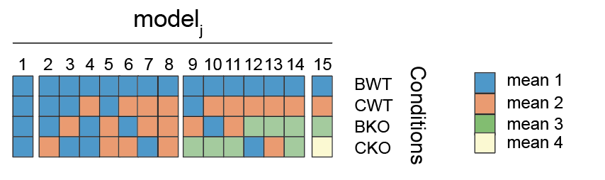
![]() is interpreted as the probability for model j. The model with the highest BIC was selected as the optimal model within the set of all defined models. In the second step, we analyzed the mean levels and thus set the coefficient
is interpreted as the probability for model j. The model with the highest BIC was selected as the optimal model within the set of all defined models. In the second step, we analyzed the mean levels and thus set the coefficient ![]() and
and ![]() to the values of the selected model in the first regression. A new regression was performed where the parameter
to the values of the selected model in the first regression. A new regression was performed where the parameter ![]() was either free or subject to constraints between conditions based on several competing models. We considered all possible combinations for the mean coefficient
was either free or subject to constraints between conditions based on several competing models. We considered all possible combinations for the mean coefficient ![]() with differing or shared means between conditions. For example, for four conditions, there are 15 such models (figure below). Each model was solved using generalized linear regression and each gene was assigned to a preferred model based on the BICW as described above for the first iteration. Cook's distance is an estimate of how much a data point influences the fitted coefficients for a gene. A large value of Cook's distance is considered to be an outlier. Thus, genes that did not reach at least one BICW above 0.4 for the preferred model or genes that had at least a Cook's distance of more than 1 were categorized as "ambiguous" (model 0). In the case of two conditions (i.e., PARbZip KO dataset) the threshold on BICW was set to 0.95. The difference in the two BICW thresholds reflected that the number of possible models is much larger for four compared to two conditions. Also, we considered only genes with a log2 amplitude of at least 0.25 to be rhythmic in the corresponding condition. To asses temporal variation of normally distributed measurements (e.g., relative liver size, nuclear abundance of PPARa), we modified model selection approach described above to deal with gaussian noise and therefore used linear models. A function handling normally distributed data is implemented in the dryR package.
with differing or shared means between conditions. For example, for four conditions, there are 15 such models (figure below). Each model was solved using generalized linear regression and each gene was assigned to a preferred model based on the BICW as described above for the first iteration. Cook's distance is an estimate of how much a data point influences the fitted coefficients for a gene. A large value of Cook's distance is considered to be an outlier. Thus, genes that did not reach at least one BICW above 0.4 for the preferred model or genes that had at least a Cook's distance of more than 1 were categorized as "ambiguous" (model 0). In the case of two conditions (i.e., PARbZip KO dataset) the threshold on BICW was set to 0.95. The difference in the two BICW thresholds reflected that the number of possible models is much larger for four compared to two conditions. Also, we considered only genes with a log2 amplitude of at least 0.25 to be rhythmic in the corresponding condition. To asses temporal variation of normally distributed measurements (e.g., relative liver size, nuclear abundance of PPARa), we modified model selection approach described above to deal with gaussian noise and therefore used linear models. A function handling normally distributed data is implemented in the dryR package.
Functional and Gene Set Enrichment Analysis
We tested enrichment for annotated gene sets of several sources including Gene Ontology [7], Molecular Signatures Database (MSigDB) [8], Kyoto Encyclopedia of Genes and Genomes (KEGG) [9] and Reactome Pathway database [10]. Target genes for circadian clock regulators and PPARa were defined as outlined below. We used GOseq 3.1 [11] to assess overrepresentation of all gene sets for genes assigned to a statistical model. Temporal resolved enrichments were calculated using a Fisher's exact test. We defined foreground genes as genes with a peak phase within in a sliding 4 h window. The gene universe was defined as all expressed genes. For each gene set the window was moved by 0.1 hr to calculate the p-value.
References
- 1. Jouffe, C., et al., Perturbed rhythmic activation of signaling pathways in mice deficient for Sterol Carrier Protein 2-dependent diurnal lipid transport and metabolism. Sci Rep, 2016. 6: p. 24631.
- 2. Gachon, F., et al., The loss of circadian PAR bZip transcription factors results in epilepsy. Genes Dev, 2004. 18(12): p. 1397-412.
- 3. Edgar, R., M. Domrachev, and A.E. Lash, Gene Expression Omnibus: NCBI gene expression and hybridization array data repository. Nucleic Acids Res, 2002. 30(1): p. 207-10.
- 4. Love, M.I., W. Huber, and S. Anders, Moderated estimation of fold change and dispersion for RNA-seq data with DESeq2. Genome Biol, 2014. 15(12): p. 550.
- 5. Anders, S. and W. Huber, Differential expression analysis for sequence count data. Genome Biol, 2010. 11(10): p. R106.
- 6. Kass, R.E. and A.E. Raftery, Bayes Factors. Journal of the American Statistical Association, 1995. 90(430): p. 773-795.
- 7. Ashburner, M., et al., Gene ontology: tool for the unification of biology. The Gene Ontology Consortium. Nat Genet, 2000. 25(1): p. 25-9.
- 8. Liberzon, A., et al., Molecular signatures database (MSigDB) 3.0. Bioinformatics, 2011. 27(12): p. 1739-40.
- 9. Kanehisa, M. and S. Goto, KEGG: kyoto encyclopedia of genes and genomes. Nucleic Acids Res, 2000. 28(1): p. 27-30.
- 10. Joshi-Tope, G., et al., Reactome: a knowledgebase of biological pathways. Nucleic Acids Res, 2005. 33(Database issue): p. D428-32.
- 11. Young, M.D., et al., Gene ontology analysis for RNA-seq: accounting for selection bias. Genome Biol, 2010. 11(2): p. R14.